Notebook01: Compute Order Parameters
Contents
Notebook01: Compute Order Parameters#
In this notebook, we’ll show you how to do the complete pipeline from downloading a united-atom trajectory file (Berger POPC) from Zenodo, reconstructing hydrogens and calculating the order parameters using buildH. In addition, we show how to plot the calculated order parameters using matplotlib.
Foreword#
Launching Unix commands within a Jupyter Notebook#
Even though buildH can be used as a module (see Notebook04), it is mainly intended to be used in the Unix command line in a terminal. Thus, many cells in this notebook will run Unix commands instead of Python instructions. All Unix commands are prefixed with the symbol !. For example:
[1]:
!ls
img
Notebook_01_buildH_calc_OP.ipynb
Notebook_02_buildH_calc_OP_outputwH.ipynb
Notebook_03_mixture_POPC_POPE.ipynb
Notebook_04_library.ipynb
Notebook_05_mixture_POPC_cholesterol.ipynb
Checking buildH installation#
First, you have to install buildH. For that you can follow the instructions on the main README of the buildH repository or the installation help page. If you did not install buildH, this notebook will not work.
Before launching this notebook, you should have activated the conda environment from buildH (the $ below corresponds to you prompt) :
$ conda activate buildh
If this command worked, you should have got the message (buildh) at the beginning of your prompt stating that the buildh environment has been properly activated.
Once done, you have launched this Jupyter notebook :
$ jupyter lab
At this point, we should be able to launch buildH within this notebook:
[2]:
!buildH
usage: buildH [-h] [-v] -c COORD [-t TRAJ] -l LIPID
              [-lt LIPID_TOPOLOGY [LIPID_TOPOLOGY ...]] -d DEFOP
              [-opx OPDBXTC] [-o OUT] [-b BEGIN] [-e END]  [-igch3]
buildH: error: the following arguments are required: -c/--coord, -l/--lipid, -d/--defop
If you do not get this usage message and have some error, you probably did not activate correctly the buildH conda environment before launching this notebook. One other possibility is that the installation of the buildH environment did not succeed. In such a case, please refer to buildH installation.
Trajectory download#
Most of the time, you will use buildH on trajectories that you have produced. Here, for the sake of learning, let us download a trajectory of a Berger POPC membrane from Zenodo (taken from NMRlipidsI project). This should take a while for the trr file, so be patient!
[3]:
!wget https://zenodo.org/record/13279/files/popc0-25ns.trr
!wget https://zenodo.org/record/13279/files/endCONF.gro
!ls
--2021-07-06 16:49:43--  https://zenodo.org/record/13279/files/popc0-25ns.trr
Resolving zenodo.org (zenodo.org)... 137.138.76.77
Connecting to zenodo.org (zenodo.org)|137.138.76.77|:443... connected.
HTTP request sent, awaiting response... 200 OK
Length: 1712544744 (1.6G) [application/octet-stream]
Saving to: ‘popc0-25ns.trr’

popc0-25ns.trr      100%[===================>]   1.59G  20.5MB/s    in 74s

2021-07-06 16:50:58 (21.9 MB/s) - ‘popc0-25ns.trr’ saved [1712544744/1712544744]

--2021-07-06 16:50:59--  https://zenodo.org/record/13279/files/endCONF.gro
Resolving zenodo.org (zenodo.org)... 137.138.76.77
Connecting to zenodo.org (zenodo.org)|137.138.76.77|:443... connected.
HTTP request sent, awaiting response... 200 OK
Length: 1968406 (1.9M) [application/octet-stream]
Saving to: ‘endCONF.gro’

endCONF.gro         100%[===================>]   1.88M  10.5MB/s    in 0.2s

2021-07-06 16:51:00 (10.5 MB/s) - ‘endCONF.gro’ saved [1968406/1968406]

endCONF.gro
img
Notebook_01_buildH_calc_OP.ipynb
Notebook_02_buildH_calc_OP_outputwH.ipynb
Notebook_03_mixture_POPC_POPE.ipynb
Notebook_04_library.ipynb
Notebook_05_mixture_POPC_cholesterol.ipynb
popc0-25ns.trr
OK the 2 files freshly downloaded are here. Now we need one last file. It’s a definition file relating generic names for each C-H bond to the atom names in the PDB file. In buildH, there is a specific directory def_files from which you can download such a def file. (note that you can find some also on the NMRlipids repo). Here we want to download the
.def file corresponding to POPC Berger :
[4]:
!wget https://raw.githubusercontent.com/patrickfuchs/buildH/master/def_files/Berger_POPC.def
!ls
--2021-07-06 16:52:18--  https://raw.githubusercontent.com/patrickfuchs/buildH/master/def_files/Berger_POPC.def
Resolving raw.githubusercontent.com (raw.githubusercontent.com)... 185.199.108.133, 185.199.109.133, 185.199.110.133, ...
Connecting to raw.githubusercontent.com (raw.githubusercontent.com)|185.199.108.133|:443... connected.
HTTP request sent, awaiting response... 200 OK
Length: 2135 (2.1K) [text/plain]
Saving to: ‘Berger_POPC.def’

Berger_POPC.def     100%[===================>]   2.08K  --.-KB/s    in 0.001s

2021-07-06 16:52:18 (3.09 MB/s) - ‘Berger_POPC.def’ saved [2135/2135]

Berger_POPC.def
endCONF.gro
img
Notebook_01_buildH_calc_OP.ipynb
Notebook_02_buildH_calc_OP_outputwH.ipynb
Notebook_03_mixture_POPC_POPE.ipynb
Notebook_04_library.ipynb
Notebook_05_mixture_POPC_cholesterol.ipynb
popc0-25ns.trr
Let us have a look to this def file:
[5]:
!head Berger_POPC.def
gamma1_1 POPC C1  H11
gamma1_2 POPC C1  H12
gamma1_3 POPC C1  H13
gamma2_1 POPC C2  H21
gamma2_2 POPC C2  H22
gamma2_3 POPC C2  H23
gamma3_1 POPC C3  H31
gamma3_2 POPC C3  H32
gamma3_3 POPC C3  H33
beta1 POPC C5  H51
The first column is the generic C-H name, second is the residue (lipid) name, third column the carbon PDB name, last column the hydrogen PDB name. This file will tell buildH which Hs you want to rebuild, and then to calculate the order parameter on the corresponding C-Hs. It means that it is possible to provide only a subset of possible C-Hs if, for example, you only want those from the polar heads. Note that if you request buildH to output a trajectory (not done in this notebook), the def file must contain all possible C-Hs of the lipid considered. In such a case, the newly built H will have the name written in the 4th column of this def file.
Now, let’s have a quick look to the .gro file:
[6]:
!head endCONF.gro
Generated by trjconv : 2:1:1 sdpc:SM:CHOL system 256 lipids t= 50000.00000
28526
    1PLA     C1    1   5.576   3.681   2.227 -0.0394  0.0935 -0.3339
    1PLA     C2    2   5.553   3.886   2.337  0.1128 -0.0058 -0.1560
    1PLA     C3    3   5.762   3.834   2.277 -0.6144  0.1201 -0.8703
    1PLA     N4    4   5.640   3.768   2.326 -0.1182 -0.1907 -0.0302
    1PLA     C5    5   5.658   3.709   2.460 -0.2986 -0.2323 -0.0245
    1PLA     C6    6   5.766   3.607   2.495  0.4136  0.5471  0.0677
    1PLA     O7    7   5.752   3.488   2.417  0.3142  0.2538  0.5323
    1PLA     P8    8   5.893   3.411   2.413  0.2220  0.1104  0.0738
We see that in this .gro file containing POPC lipids, the residue name is called PLA. This residue name will be of importance when launching buildH.
Great, all files were successfully downloaded, we can now proceed. Let us launch buildH!
Launching buildH for order parameter calculation#
Now, we can launch buildH on this downloaded trajectory. For that we need a few arguments :
the
-cargument corresponding to the coordinate file. It consists of a pdb or gro file, hereendCONF.gro, buildH infers the topology of the system from it;the
-largument which tells which lipid we want to analyze, hereBerger_PLA(Bergercorresponds to the force field name used for this simulation,PLAis the residue name of the lipid we want to analyze in the pdb/gro file); note that if you simulated a mixture of different lipids, you will have to launch buildH separately for each lipid (see Notebook03 and Notebook05);the
-dargument corresponding to the def file we just downloaded, hereBerger_POPC.def;the
-targument which is the trajectory file, herepopc0-25ns.trr.the
-oargument which tells buildH the output file name for storing the calculated order parameters.
Please be patient, this will take a while since we have 2500 frames. Fortunately, buildH geometrical calculations are accelerated using Numba. On single core Xeon @ 3.60GHz, it took ~ 7’.
[7]:
!buildH -c endCONF.gro -l Berger_PLA -d Berger_POPC.def -t popc0-25ns.trr -o OP_POPC_Berger_25ns.out
Constructing the system...
System has 28526 atoms
Dealing with frame 0 at 0.0 ps.
Dealing with frame 1 at 10.0 ps.
Dealing with frame 2 at 20.0 ps.
Dealing with frame 3 at 30.0 ps.
Dealing with frame 4 at 40.0 ps.
Dealing with frame 5 at 50.0 ps.
Dealing with frame 6 at 60.0 ps.
Dealing with frame 7 at 70.0 ps.
Dealing with frame 8 at 80.0 ps.
Dealing with frame 9 at 90.0 ps.
Dealing with frame 10 at 100.0 ps.
Dealing with frame 11 at 110.0 ps.
Dealing with frame 12 at 120.0 ps.
Dealing with frame 13 at 130.0 ps.
Dealing with frame 14 at 140.0 ps.
Dealing with frame 15 at 150.0 ps.
Dealing with frame 16 at 160.0 ps.
Dealing with frame 17 at 170.0 ps.
Dealing with frame 18 at 180.0 ps.
Dealing with frame 19 at 190.0 ps.
Dealing with frame 20 at 200.0 ps.
Dealing with frame 21 at 210.0 ps.
Dealing with frame 22 at 220.0 ps.
^C
Traceback (most recent call last):
  File "/home/fuchs/software/miniconda3/envs/buildh/bin/buildH", line 33, in <module>
    sys.exit(load_entry_point('buildh', 'console_scripts', 'buildH')())
  File "/home/fuchs/papers/buildH_project/buildH/buildh/UI.py", line 148, in entry_point
    main(args.coord, args.traj, args.defop, args.out, args.opdbxtc, dic_lipid, args.begin, args.end)
  File "/home/fuchs/papers/buildH_project/buildH/buildh/UI.py", line 341, in main
    core.fast_build_all_Hs_calc_OP(universe_woH, begin, end, dic_OP,
  File "/home/fuchs/papers/buildH_project/buildH/buildh/core.py", line 533, in fast_build_all_Hs_calc_OP
    Hs_coor = buildHs_on_1C(Cname_position, typeofH2build,
  File "/home/fuchs/papers/buildH_project/buildH/buildh/core.py", line 59, in buildHs_on_1C
    H1_coor, H2_coor, H3_coor = hydrogens.get_CH3(atom,
  File "/home/fuchs/papers/buildH_project/buildH/buildh/hydrogens.py", line 114, in get_CH3
    coor_He = LENGTH_CH_BOND * unit_vect_He + atom
KeyboardInterrupt
On the above cell, we launched buildH to show you how it works. For each frame handled by buildH, a message Dealing with frame XXX at YYY ps. is printed to the output. Because it takes some time and because it should have printed 2500 Dealing with frame..., we just pressed Ctrl-C to get this notebook not too much polluted by buildH output. This explains why there is a Python KeyboardInterrupt message.
Note that, you can also launch buildH in a regular shell that way:
$ buildH -c endCONF.gro -l Berger_PLA -d Berger_POPC.def -t popc0-25ns.trr -o OP_POPC_Berger_25ns.out
Or that way:
$ buildH -c endCONF.gro -l Berger_PLA -d Berger_POPC.def -t popc0-25ns.trr -o OP_POPC_Berger_25ns.out > /dev/null
In this case, all the messages Dealing with frame... go to /dev/null, thus no more lengthy output ;-)
Once completed, we should have a new file called OP_POPC_Berger_25ns.out containing the order parameters. You can choose any name with the option -o when you launch buildH. If you did not run buildH on the full trajectory, you can find that file here.
[9]:
!ls
Berger_POPC.def
endCONF.gro
img
Notebook_01_buildH_calc_OP.ipynb
Notebook_02_buildH_calc_OP_outputwH.ipynb
Notebook_03_mixture_POPC_POPE.ipynb
Notebook_04_library.ipynb
Notebook_05_mixture_POPC_cholesterol.ipynb
OP_POPC_Berger_25ns.out
popc0-25ns.trr
Analyzing results#
First, let’s have a look to what this output file OP_POPC_Berger_25ns.out contains.
[10]:
!head OP_POPC_Berger_25ns.out
# OP_name            resname atom1 atom2  OP_mean OP_stddev OP_stem
#--------------------------------------------------------------------
gamma1_1             PLA     C1    H11    0.01788  0.09262  0.00819
gamma1_2             PLA     C1    H12   -0.00744  0.03963  0.00350
gamma1_3             PLA     C1    H13   -0.00855  0.03601  0.00318
gamma2_1             PLA     C2    H21    0.01850  0.09283  0.00820
gamma2_2             PLA     C2    H22   -0.00666  0.04559  0.00403
gamma2_3             PLA     C2    H23   -0.00894  0.04016  0.00355
gamma3_1             PLA     C3    H31    0.01854  0.09235  0.00816
gamma3_2             PLA     C3    H32   -0.01158  0.03796  0.00335
For each C-H we get the mean order parameter OP_mean (average over frames and over residues), its standard deviation OP_stddev (standard deviation over residues), and its standard error of the mean OP_stem (OP_stddev divided by the square root of the number of residues). More information about how OP_mean, OP_stddev and OP_stem are computed can be found in the documentation: Order parameters and statistics
Now we can make a plot of the order parameter. For that, we can use Pandas and its very convenient dataframes to load buildH output. Pandas dataframes allow the selection of any row or column in a very powerful way. If you are not familiar with pandas dataframes, you can take a look here. For reading buildH output and
generate a dataframe, we use the Pandas function .read_csv() which has a great deal of options to read a file. Here we tell it to use a specific separator (\s+ which means any combination of white spaces), to skip 2 lines at the beginning of the files (beginning with a #) and to assign specific names to each column.
[11]:
import pandas as pd

df = pd.read_csv("OP_POPC_Berger_25ns.out", sep="\s+", skiprows=2,
                 names=["CH_name", "res", "carbon", "hydrogen", "OP", "STD", "STEM"])
df
[11]:
| CH_name | res | carbon | hydrogen | OP | STD | STEM | |
|---|---|---|---|---|---|---|---|
| 0 | gamma1_1 | PLA | C1 | H11 | 0.01788 | 0.09262 | 0.00819 |
| 1 | gamma1_2 | PLA | C1 | H12 | -0.00744 | 0.03963 | 0.00350 |
| 2 | gamma1_3 | PLA | C1 | H13 | -0.00855 | 0.03601 | 0.00318 |
| 3 | gamma2_1 | PLA | C2 | H21 | 0.01850 | 0.09283 | 0.00820 |
| 4 | gamma2_2 | PLA | C2 | H22 | -0.00666 | 0.04559 | 0.00403 |
| ... | ... | ... | ... | ... | ... | ... | ... |
| 77 | oleoyl_C17a | PLA | CA1 | HA11 | -0.05500 | 0.01999 | 0.00177 |
| 78 | oleoyl_C17b | PLA | CA1 | HA12 | -0.05225 | 0.01950 | 0.00172 |
| 79 | oleoyl_C18a | PLA | CA2 | HA21 | 0.03903 | 0.02647 | 0.00234 |
| 80 | oleoyl_C18b | PLA | CA2 | HA22 | -0.05292 | 0.02033 | 0.00180 |
| 81 | oleoyl_C18c | PLA | CA2 | HA23 | -0.05025 | 0.01972 | 0.00174 |
82 rows × 7 columns
If we want only the order parameter for the polar head we can use the following. Suffixing the dataframe with a list of lists [["CH_name", "OP"]] allows us to select the columns we are interested in. Then, with the .iloc() method we can get the 18 first rows corresponding to the polar head (beware it starts counting at 0 like all sequential objects in Python).
[12]:
df[["CH_name", "OP"]].iloc[:18]
[12]:
| CH_name | OP | |
|---|---|---|
| 0 | gamma1_1 | 0.01788 |
| 1 | gamma1_2 | -0.00744 |
| 2 | gamma1_3 | -0.00855 |
| 3 | gamma2_1 | 0.01850 |
| 4 | gamma2_2 | -0.00666 |
| 5 | gamma2_3 | -0.00894 |
| 6 | gamma3_1 | 0.01854 |
| 7 | gamma3_2 | -0.01158 |
| 8 | gamma3_3 | -0.00715 |
| 9 | beta1 | 0.03634 |
| 10 | beta2 | 0.06587 |
| 11 | alpha1 | 0.10349 |
| 12 | alpha2 | 0.13568 |
| 13 | g3_1 | -0.28403 |
| 14 | g3_2 | -0.15962 |
| 15 | g2_1 | -0.16767 |
| 16 | g1_1 | 0.20330 |
| 17 | g1_2 | 0.08910 |
Let us do the same for the palmitoyl chain.
[13]:
df[["CH_name", "OP"]].iloc[18:49]
[13]:
| CH_name | OP | |
|---|---|---|
| 18 | palmitoyl_C2a | -0.17593 |
| 19 | palmitoyl_C2b | -0.16136 |
| 20 | palmitoyl_C3a | -0.19742 |
| 21 | palmitoyl_C3b | -0.18853 |
| 22 | palmitoyl_C4a | -0.19367 |
| 23 | palmitoyl_C4b | -0.18011 |
| 24 | palmitoyl_C5a | -0.19815 |
| 25 | palmitoyl_C5b | -0.19364 |
| 26 | palmitoyl_C6a | -0.19251 |
| 27 | palmitoyl_C6b | -0.19193 |
| 28 | palmitoyl_C7a | -0.18894 |
| 29 | palmitoyl_C7b | -0.19106 |
| 30 | palmitoyl_C8a | -0.17809 |
| 31 | palmitoyl_C8b | -0.17827 |
| 32 | palmitoyl_C9a | -0.17190 |
| 33 | palmitoyl_C9b | -0.17066 |
| 34 | palmitoyl_C10a | -0.15468 |
| 35 | palmitoyl_C10b | -0.15328 |
| 36 | palmitoyl_C11a | -0.14349 |
| 37 | palmitoyl_C11b | -0.14297 |
| 38 | palmitoyl_C12a | -0.12392 |
| 39 | palmitoyl_C12b | -0.12448 |
| 40 | palmitoyl_C13a | -0.11173 |
| 41 | palmitoyl_C13b | -0.11094 |
| 42 | palmitoyl_C14a | -0.09097 |
| 43 | palmitoyl_C14b | -0.09039 |
| 44 | palmitoyl_C15a | -0.07367 |
| 45 | palmitoyl_C15b | -0.07496 |
| 46 | palmitoyl_C16a | 0.11169 |
| 47 | palmitoyl_C16b | -0.07181 |
| 48 | palmitoyl_C16c | -0.07307 |
And now, for the oleoyl chain.
[14]:
df[["CH_name", "OP"]].iloc[49:]
[14]:
| CH_name | OP | |
|---|---|---|
| 49 | oleoyl_C2a | -0.15474 |
| 50 | oleoyl_C2b | -0.17336 |
| 51 | oleoyl_C3a | -0.16911 |
| 52 | oleoyl_C3b | -0.17847 |
| 53 | oleoyl_C4a | -0.17385 |
| 54 | oleoyl_C4b | -0.18235 |
| 55 | oleoyl_C5a | -0.17504 |
| 56 | oleoyl_C5b | -0.17690 |
| 57 | oleoyl_C6a | -0.16138 |
| 58 | oleoyl_C6b | -0.16692 |
| 59 | oleoyl_C7a | -0.15512 |
| 60 | oleoyl_C7b | -0.15994 |
| 61 | oleoyl_C8a | -0.10190 |
| 62 | oleoyl_C8b | -0.10603 |
| 63 | oleoyl_C9a | -0.08281 |
| 64 | oleoyl_C10a | -0.01791 |
| 65 | oleoyl_C11a | -0.05119 |
| 66 | oleoyl_C11b | -0.04599 |
| 67 | oleoyl_C12a | -0.09275 |
| 68 | oleoyl_C12b | -0.08879 |
| 69 | oleoyl_C13a | -0.08643 |
| 70 | oleoyl_C13b | -0.08259 |
| 71 | oleoyl_C14a | -0.09133 |
| 72 | oleoyl_C14b | -0.08893 |
| 73 | oleoyl_C15a | -0.07729 |
| 74 | oleoyl_C15b | -0.07524 |
| 75 | oleoyl_C16a | -0.07256 |
| 76 | oleoyl_C16b | -0.07041 |
| 77 | oleoyl_C17a | -0.05500 |
| 78 | oleoyl_C17b | -0.05225 |
| 79 | oleoyl_C18a | 0.03903 |
| 80 | oleoyl_C18b | -0.05292 |
| 81 | oleoyl_C18c | -0.05025 |
Plot of the order parameter#
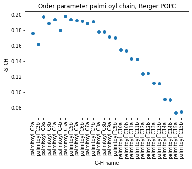
Now that we have loaded the data with pandas, and that we can select any part of the lipid, we can use the matplotlib module to make a nice plot. For example, we can plot the order parameter of the palmitoyl chain. Note that we select rows 18 to 45 to show only the first 15 carbons, since we do not want the final CH3 of carbon 16.
[15]:
import numpy as np
import matplotlib.pyplot as plt

OPs = df["OP"].iloc[18:46]

x = np.arange(len(OPs))
plt.scatter(x, -OPs)
plt.xticks(x, df["CH_name"].iloc[18:46], rotation='vertical')
plt.xlabel("C-H name")
plt.ylabel("-S_CH")
plt.title("Order parameter palmitoyl chain, Berger POPC")
[15]:
Text(0.5, 1.0, 'Order parameter palmitoyl chain, Berger POPC')
Another example with the polar head, on the alpha beta of the choline and glycerol C-Hs.
[16]:
import numpy as np
import matplotlib.pyplot as plt

OPs = df["OP"].iloc[9:18]
STEMs = df["STEM"].iloc[9:18]

# These 2 avoid plotting a line between the points.
lines = {'linestyle': 'None'}
plt.rc('lines', **lines)

x = np.arange(len(OPs))
plt.errorbar(x, -OPs, STEMs, fmt='', marker='.')
plt.xticks(x, df["CH_name"].iloc[9:18], rotation='vertical')
plt.xlabel("C-H name")
plt.ylabel("-S_CH")
plt.title("Order parameter polar head, Berger POPC")
[16]:
Text(0.5, 1.0, 'Order parameter polar head, Berger POPC')
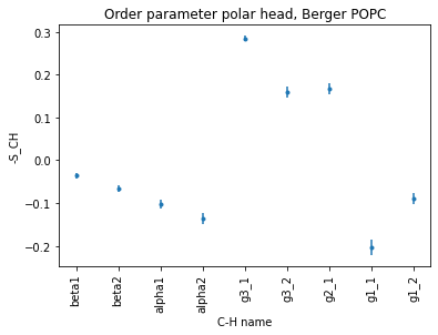
Since the error bars are very small, we used marker='.' to draw tiny points. If we use the standard marker='o', the error bars are often not seen because they are smaller than the point itself.
Conclusion#
In this notebook, we showed you how to use buildH to build hydrogens from a united-atom trajectory and calculate the order parameter on it. Then, we showed some convenient use of pandas and matplotlib Python modules to select the data we are interested in and plot the corresponding results.